Portfolio Optimization: Minimize risk with Turnover constraint via Quadratic Programming

Rebalancing portfolios is an important event in the life of the portfolio manager, whether we talk about the timing or the degree of the rebalancing, i.e. the portfolio turnover, this is a sensitive operation. As well as the first one is important to avoid bad timing market effects, the second one has direct implication on friction costs, a.k.a the transactions costs.

In this article, we will focus on mitigating the latter one, i.e. control the portfolio turnover when adjusting your fund’s positions.

We shall take an initial hypothetical equity portfolio x₀, of N stocks. Our quantitative model was executed and now presents us a new portfolio x₁ (same universe of stocks). However the turnover between x₀ and x₁ is around 10%, and in our portfolio management process, we have a maximum turnover constraint of 5%. To satisfy both needs (rebalance to keep following strategy’s signal and lower turnover to mitigate transaction fees), we will apply an optimization, to find the optimal portfolio x.

We define the turnover ratio τ as the absolute sum of the sales and purchases between x₀ and x.

\tau= \sum\limits_{i=1}^N{|x_{i}-x_{0,i}|}

Our objective will be to minimize the tracking error between the current portfolio and the target portfolio, with a linear constraint on turnover. The idea here, is to find the optimal portfolio that is the closest to our target portfolio but close enough to the old one, to respect our turnover requirement of 5%.

The interest of formulating this problem as a Quadratic Progamming problem is to benefit from the convex optimization framework⁽¹⁾, i.e. be sure that the solution will be the global minimum.

Now let’s define our quadratic programming (QP) problem.

The standard QP problem can be written as:

minimize:\; \frac{1}{2}x^\top Px+q^\top x \\
subject\:to:\; 
\left\{
\begin{array}{ll}
Gx\leqslant h \\
Ax=b
\end{array}
 \right.

Here we want to obtain an unleveraged long-only portfolio, with a maximum turnover constraint τ⁺ (5% in our example). We will be using a stocks’ returns covariance matrix named Σ.

Consequently, the QP problem now becomes:

minimize:\; \frac{1}{2}x^\top\Sigma x-x_{1}^\top\Sigma x \\
subject\:to:\;  
\left\{
\begin{array}{ll}
\sum\limits_{i=1}^N{x_{i}} = 1 \\
\sum\limits_{i=1}^N{|x_{i}-x_{0,i}|} \leqslant \tau^+\\
0 \leqslant x_i \leqslant 1 , \; with \, i \in [1,N]
\end{array}
 \right.

However, we can’t feed directly our QP solver with this problem, as the turnover constraint is not compatible. First, we should transform this 1N-dimensional QP problem to a higher dimensional QP problem.

Thanks to the introduction of two additional variables x_i⁺ and x_i^–, both positives, representing respectively the purchases and the sales between x₀ and x, we can rewrite the turnover definition.

x_i = x_{0,i} + x_i^+ - x_i^-  , \; with \, i \in [1,N] \\
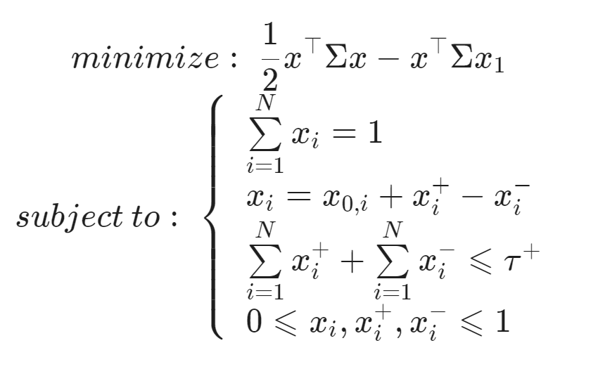
\tau = \sum\limits_{i=1}^N{|x_{i}-x_{0,i}|} = \sum\limits_{i=1}^N{|x_i^+ -x_i^- |} = \sum\limits_{i=1}^N{x_i^+} + \sum\limits_{i=1}^N{x_i^-} 

We now have the following 3N-dimensional QP problem.

minimize:\; \frac{1}{2}x^\top\Sigma x-x_{1}^\top\Sigma x \\
subject\:to:\;  
\left\{
\begin{array}{ll}
\sum\limits_{i=1}^N{x_{i}} = 1 \\
x_i = x_{0,i} + x_i^+ - x_i^- , \; with \, i \in [1,N] \\
\sum\limits_{i=1}^N{x_i^+} + \sum\limits_{i=1}^N{x_i^-} \leqslant \tau^+\\

0 \leqslant x_i,x_i^+,x_i^- \leqslant 1 , \; with \, i \in [1,N]
\end{array}
 \right.

Using the standard QP formulation, we can write this augmented QP problem in matrix notation⁽²⁾.

P = 
\begin{pmatrix}
\Sigma & 0_{N \times N} & 0_{N \times N} \\
0_{N \times N} & 0_{N \times N} & 0_{N \times N} \\
0_{N \times N} & 0_{N \times N} & 0_{N \times N}
\end{pmatrix} \\ 
q = 
\begin{pmatrix}
-\Sigma x_1 & 0_{N} & 0_{N}
\end{pmatrix} \\
A = 
\begin{pmatrix}
1_{N}^\top & 0_{N}^\top & 0_{N}^\top \\
I_{N} & I_{N}& -I_{N}
\end{pmatrix} \\
b = (1,x_0) \\
G = 
\begin{pmatrix}
0_{N}^\top & 1_{N}^\top & 1_{N}^\top \\
-I_{N} & 0_{N \times N} & 0_{N \times N} \\
0_{N \times N} & -I_{N} & 0_{N \times N} \\
0_{N \times N} & 0_{N \times N} & -I_{N}
\end{pmatrix} \\
h = (\tau^+, 0_{3N \times 1})

Now let’s look at the code to compute this.

First thing, we import our libraries. We will be using the cvxopt library for the convex solver.

import numpy as np
from cvxopt import solvers, matrix

Then we import the data to be used, i.e. covariance matrix, and weights of portfolios x₀ and x₁.

cov = '...' # load covariance matrix (NxN)
x0 = '...' # load current portfolio x0 (size N)
x1 = '...' # load target portfolio x1 (size N)
turnover_constraint = 0.05 # 5% max turnover
N = len(cov)

Now let’s define our vectors & matrices P, q, A, b, G, h (from the formulation written above).

# define P & q
P = matrix(np.block([[np.array(cov), 0*np.array(cov), 0*np.array(cov)],
           [0*np.array(cov), 0*np.array(cov), 0*np.array(cov)],
           [0*np.array(cov), 0*np.array(cov), 0*np.array(cov)]]))

q = matrix(np.block([-cov.dot(x1), np.zeros((N)), np.zeros((N))]))     

# equalities constraints   
A = matrix(np.block([[np.ones(N).T, np.zeros(N).T, np.zeros(N).T],
                    [np.eye(N),np.eye(N),-np.eye(N)]]))
b = matrix(np.block([1,x0.T]))     

# inequalities constraints    
G = matrix(np.block([[np.zeros(N).T,np.ones(N).T,np.ones(N).T],
                    [-np.eye(N),np.zeros((N,N)),np.zeros((N,N))],
                    [np.zeros((N,N)),-np.eye(N),np.zeros((N,N))],
                    [np.zeros((N,N)),np.zeros((N,N)),-np.eye(N)]]))     
h = matrix(np.concatenate((np.ones((1,1))*turnover_constraint, np.zeros((3*N,1))), axis=0))

# solve problem
result = solvers.qp(P,q,G,h,A,b)

# store optimization result's status
status = result['status']

# store optimal portfolio
x_optimal = np.array(result['x'])[0:N]

# store tracking-error of optimal portfolio x versus target portfolio x1
result_tracking_error = np.sqrt((x_optimal.reshape(len(x_optimal)) -x1).T.dot(cov).dot((x_optimal.reshape(len(x_optimal)) - x1)))   

# store turnover ratio between optimal portfolio x and previous portfolio x0
result_turnover = np.abs(x_optimal.reshape(len(x_optimal)) - x0).sum()

To conclude, in this study, we formulated a tracking-error minimization problem under a linear constraint of turnover, as a QP problem, which allowed us to obtain a global minimum solution. This is really helpful to get a trade-off between following closely your strategy’s signal and mitigating transaction fees, when rebalancing your portfolio.

Remarks
(1) As covariance matrices are usually positive-definite, the QP problem becomes a special case of convex optimization.
(2) Here no need to write x_i, x_i⁺​ or x_i⁻​⩽1​, as it is induced by the other constraints.

References
S. Perrin, T. Roncalli (2019), Machine Learning Optimization Algorithms & Portfolio Allocation, arXiv:1909.10233.