Portfolio Optimization: Replicate a corporate bond index via Mixed-Integer Programming
While portfolio optimization is well known in the Equity space, in the Fixed Income industry, the subject is less discussed although it has very specific needs and it can be more complex compared to its Equity counterparts. One key difference between the two of them is the trading lot size.
In Equities, most of the time, you can generate a portfolio composition directly with weights (continous data) and not a number of holdings (discretionary data). Implementing the real portfolio by transforming weights into holdings is easy thanks to lot sizes which are usually quite low, the delta between model and resulting real portfolio is negligible.
In Fixed Income, and more precisely on our area of interest, corporate bonds, the story is quite different. You can’t trade like for equities only 1 share of the asset, you have what is called a minimum tradable (the minimum amount for which you can trade a bond, a.k.a. minimum denomination) and a minimum increment (the minimum lot size you can add up). For example a bond with a min tradable of 100k€ and a min increment of 100k€, you can’t trade 150k€ of this bond, you have to buy either 100 or 200k€ of it. For large funds (>2 or 3 billions €) you won’t have big problems (as a smart rounding process could be sufficient), but for smaller funds (100M€, 500M€) you can encounter some difficulties when optimizing by weights.
In the case of the replication of an index, a 100% physical replication like for equity ETFs is rarely possible due to this size effect. In this extent, replicating through sampling is often mandatory. Like for equities, the objective would be to minimize the tracking error between the model portfolio and the index but also add constraints to control some sensitivities and exposures, like modified duration (MD), duration times spread (DTS), liquidity (LQY), rating or sectors to only name a few ones. It is important to add these constraints as covariance matrices are less reliable on the fixed income side, and including some “guardrails” allows us to be more confident if a market shock happens.
The idea here is to formulate the optimization process as a Mixed Integer Programming (MIP) problem, or more precisely here, as a Mixed Integer Quadratic Programming (MIQP) problem. Thanks to this program, we will be able to obtain the optimal solution in terms of integer values (the holding quantities).(1)
Some libraries and solvers allow users to write (in a natural mathematical way) their problem and solve it in only a few lines of code. Here we will use the cvxpy library for the modeling part of the problem and the commercial solver XPRESS (a free version is available) to get our solution.
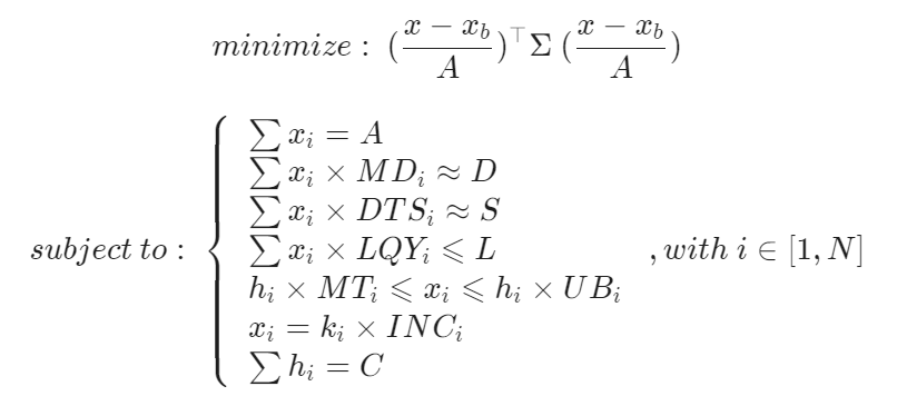
First let’s define our MIP problem, with some of the described constraints:
minimize :\ (\frac{x-x_b}{A})^\top  \Sigma\ (\frac{x-x_b}{A}) \\
 {}\\
subject\:to:\;
\left\{
\begin{array}{ll}
\sum x_i = A \\
\sum x_i \times MD_i \approx D \\
\sum x_i \times DTS_i \approx S \\
\sum x_i \times LQY_i \leqslant L \\

h_i \times MT_i \leqslant x_i \leqslant h_i \times UB_i \\
x_i = k_i \times INC_i \\
\sum h_i = C \\
\end{array}
 \right.
, with \ i \in [1, N]- A being the total par value of the resultant portfolio
- D and MDi being resp. the MD amount target of the index and bonds’ MD
- S and DTSi being resp. the DTS amount target of the index and bonds’ DTS
- L and LQYi being resp. the liquidity target of the index and bonds’ liquidity scores (the lower, the more liquid it is)
- MTi being the minimum tradable of the bonds
- INCi being the minimum increment of the bonds
- UBi being the upper bound of bonds’ holdings
- C being the number of bonds we want to hold
- xi being the par value of bonds in the resultant portfolio
- xb,i being the par value of bonds in the index
- Σ being the covariance matrix of bonds (size NxN)
- hi is a boolean variable (0 or 1)
- ki is an integer variable
- N being the number of bonds in universe
Now let’s code it! Starting with a 100% cash portfolio worth of 500M€ (of par value to invest in), from a universe of 2000 corporate bonds, let’s say we want to buy only 1000 of those bonds and keep close to the original index.
import pandas as pd
import numpy as np
import cvxpy as cvx

# load data
universe = pd.read_csv('my_data.csv')
cov = pd.read_csv('my_cov_data.csv')

# parameters
A = 50e7
N = 2000
C = 1000

# create variables to solve
x = cvx.Variable((N,1), integer=True)
h = cvx.Variable((N,1), boolean=True)
k = cvx.Variable((N,1), integer=True)

# write the constraints
constraints = [
# Total amount constraint
cvx.sum(x) == A,
# Liquidity constraint
cvx.sum(x.T @ universe.liquidity) <= (target_liquidity),
# MD constraint
cvx.sum(x.T @ universe.md) <= (target_md) * (1.0001),
cvx.sum(x.T @ universe.md) >= (target_md)  * (0.9999),
# DTS constraint
cvx.sum(x.T @ universe.dts) <= (target_dts)  * (1.0001),
cvx.sum(x.T @ universe.dts) >= (target_dts)  * (0.9999),
# Cardinality constraint
cvx.sum(h) == C,
# Min increment constraint
x == cvx.multiply(k, universe.min_x_inc.values.reshape(N,1)),
# Upper bound constraint
x <= cvx.multiply(universe.upper_bound.values.reshape(N,1), h),
# Min tradable constraint
x >= cvx.multiply(universe.min_x.values.reshape(N,1),h)
]

# write objective function
objective = cvx.Minimize(cvx.quad_form((x-universe.x_bench.values.reshape(N,1))/A, cov.values))

# create the problem
prob = cvx.Problem(objective, constraints)

# solve it
prob.solve(verbose=False, solver="XPRESS")

# store results
universe['PAR_VALUE'] = x.value
universe['INVESTED_IN'] = h.value
universe['MIN_INCR_MULTIPLE'] = k.value
We then check the characteristics of the resultant portfolio versus the index:
PTF vs Index
============
Liquidity Score: 6.941895149937941 vs 6.992608995220758
MD Score: 5.2056202113335965 vs 5.2051992581035496
DTS Score: 4.927243333700834 vs 4.927114810448214
Total bonds in PTF: 1000
Total Amount: 500000000.0
Tracking-Error ex-ante: 0.003767393032262377
To conclude, the interest of using this kind of optimization technique is that it can be easily modified to change either the objective function (mean variance, score max/min, etc.) or the constraints(2). Another key element is its great scalability to the level of notional of your portfolio, as most of the time, portfolios are not worth billions “but only” a few hundred millions (or less), therefore optimizing “classically” by weights produces results far too imprecise.
(1) Alternative methods, such as genetic algorithms, could also be applied in this situation.
(2) Rmk: Depending on the data structure and the constraints tightness, you will sometimes have to relax some of them if they make the problem infeasible to solve.