Enhance your portfolio analysis framework with carbon emissions attributions
As a portfolio manager, of a mutual or dedicated fund, you have to regularly report the performance of your fund on a specific time frame (monthly, quarterly, yearly, etc.).
One of the common tools is the performance attribution analysis, which is a framework that allows to isolate the effect between allocation and selection processes. Several methods can be used (Brinson, Top-Down, Geometric, Risk attribution, etc.), and this analysis is well spread and integrated in portfolio management frameworks.
Nowadays, ESG reporting became mandatory in lots of countries. The portfolio manager, in addition to his fiduciary duty, has to respond of its ESG policy and its implementation in its fund.
Here we will transpose this kind of methodology to analyze the carbon emissions of a portfolio.
First a quick definition of carbon emissions. It is measured in tons of Co2 (or Co2 equivalent) emitted by the company (and usually reported by the company itself once a year). This score is divided in 3 categories called “scope”.
- Scope 1 reflects direct emissions: transportation, production (manufacturing, heating, cooling, etc.).
- Scope 2 includes indirect energy emissions. This will depend on the infrastructure of the energy supplier (nuclear, coal, wind, photovoltaic, blended, etc.).
- Scope 3 captures all of the remaining indirect emissions, which is a very broad scope and very difficult to collect (investments, wastes, employees travels, product use and end of life, etc.).
Remark: Scope 3 can overlap scopes 1 & 2 of other companies. Therefore to aggregate total emissions of several companies we usually use the sum of scope 1 & 2.
Lastly, as companies have different sizes (e.g. Apple versus a family grocery store), we normalize the carbon emission by either companies sales or market cap, to produce a carbon intensity score.
Now let’s go back into the skin of the portfolio manager. It can be useful to know if your fund over/under emissions (versus a benchmark) is due to your selection or allocation processes. The difference with a performance attribution is that we analyze a portfolio composition at a spot date compared to the classic timeframe performance attribution analysis.
From a classic 2-factor performance attribution framework we can derive a carbon model. Similarly to Brinson, we choose a grouping (sector, industry, country, currency, etc.) and apply the following formulas:
Allocation\,\,impact_g = (w_{ptf,g}-w_{bench,g}) \times (Bench\_intensity_g - Bench\_intensity)
\\
Selection\,\,impact_g = w_{ptf,g} \times (Ptf\_intensity_g - Bench\_intensity_g)
Let’s dig into the metric that will be used to measure the carbon intensity.
Portfolio\,\,intensity = \sum_g{Grouping\,intensity_g \times w_g}Grouping\,\,intensity = \frac{\sum_i{w_i \times emissions_i}}{\sum_i{w_i \times sales_i}}Now let’s see the code.
import pandas as pd
import numpy as np
We create the function that computes the weighted contribution of a group to a specific metric.
def compute_contrib(df, grouping="SECTOR", ptf="PTF", score="SCOPE1+2", rebase=True):
    if rebase == True:
        return df.groupby(grouping).apply(lambda x: (x[ptf+"_WEIGHT"] * x[score] / x[ptf+"_WEIGHT"].sum()).sum())#.reset_index().set_index("level_1")[0]
    else:
        return df.groupby(grouping).apply(lambda x: (x[ptf+"_WEIGHT"] * x[score]).sum())#.reset_index().set_index("level_1")[0]
Then we create the function that generates and format the carbon attribution table.
def compute_carbon_attribution(portfolio, grouping='SECTOR', carbon_metric='SCOPE1+2', norm_metric='SALES'):
    """ Given a universe with portfolio and benchmark weights, calculate a carbon attribution based on the grouping choice (SECTOR, INDUSTRY) and carbon metric (SCOPE1, SCOPE2 or SCOPE1+2).
    The chosen carbon metric will be normalized by the normalization metric (SALES, MKTCAP).
    The attribution makes it possible to highlight the impacts of the allocation and the selection on the overall rating of the portfolio."""
    # group portfolio
    attrib = portfolio.groupby(grouping)[["PTF_WEIGHT", "BENCH_WEIGHT", "ACTIVE_WEIGHT"]].sum()
    attrib["PTF_INTENSITY"] = compute_contrib(df=portfolio, grouping=grouping, ptf="PTF", score=carbon_metric, rebase=True) / compute_contrib(df=portfolio, grouping=grouping, ptf="PTF", score=norm_metric, rebase=True)
    attrib["BENCH_INTENSITY"] = compute_contrib(df=portfolio, grouping=grouping, ptf="BENCH", score=carbon_metric, rebase=True) / compute_contrib(df=portfolio, grouping=grouping, ptf="BENCH", score=norm_metric, rebase=True)
    attrib["INTENSITY_DIFFERENCE"] = attrib["PTF_INTENSITY"] - attrib["BENCH_INTENSITY"]
    # divide between allocation and selection effects
    attrib["ALLOCATION_IMPACT"] = attrib["ACTIVE_WEIGHT"] * (attrib["BENCH_INTENSITY"] - (attrib.BENCH_WEIGHT * attrib["BENCH_INTENSITY"]).sum() )
    attrib["SELECTION_IMPACT"] = attrib["PTF_WEIGHT"] * (attrib["PTF_INTENSITY"] - attrib["BENCH_INTENSITY"])
    # add total numbers
    attrib.loc["TOTAL", "PTF_WEIGHT"] =  attrib.PTF_WEIGHT.sum()
    attrib.loc["TOTAL", "BENCH_WEIGHT"] =  attrib.BENCH_WEIGHT.sum()
    attrib.loc["TOTAL", "ACTIVE_WEIGHT"] =  attrib.ACTIVE_WEIGHT.sum()
    attrib.loc["TOTAL", "PTF_INTENSITY"] =  (attrib.PTF_WEIGHT * attrib["PTF_INTENSITY"]).sum()
    attrib.loc["TOTAL", "BENCH_INTENSITY"] =  (attrib.BENCH_WEIGHT * attrib["BENCH_INTENSITY"]).sum()
    attrib.loc["TOTAL", "INTENSITY_DIFFERENCE"] =  attrib.loc["TOTAL", "PTF_INTENSITY"] - attrib.loc["TOTAL", "BENCH_INTENSITY"]
    attrib.loc["TOTAL", "ALLOCATION_IMPACT"] =  attrib.ALLOCATION_IMPACT.sum()
    attrib.loc["TOTAL", "SELECTION_IMPACT"] =  attrib.SELECTION_IMPACT.sum()
    # scale weights to 100%
    attrib.loc[:,["PTF_WEIGHT", "BENCH_WEIGHT", "ACTIVE_WEIGHT"]] = attrib.loc[:,["PTF_WEIGHT", "BENCH_WEIGHT", "ACTIVE_WEIGHT"]] * 100
    # formatting output
    idx = pd.IndexSlice
    return attrib.style.format('{:.2f}', na_rep="")\
    .bar(subset=idx[attrib.loc[(attrib['ACTIVE_WEIGHT']>=0)].index, 'ACTIVE_WEIGHT'], color='lightpink', align=0, height=50, width=60, vmin=-50, vmax=50)\
    .bar(subset=idx[attrib.loc[(attrib['ACTIVE_WEIGHT']<0)].index, 'ACTIVE_WEIGHT'], color='lightblue', align=0, height=50, width=60, vmin=-50, vmax=50)\
    .bar(subset=idx[attrib.loc[(attrib['INTENSITY_DIFFERENCE']>=0)].index, 'INTENSITY_DIFFERENCE'], color='red', align=0, height=50, width=60, vmin=-200, vmax=200)\
    .bar(subset=idx[attrib.loc[(attrib['INTENSITY_DIFFERENCE']<0)].index, 'INTENSITY_DIFFERENCE'], color='green', align=0, height=50, width=60, vmin=-200, vmax=200)\
    .bar(subset=idx[attrib.loc[(attrib['ALLOCATION_IMPACT']>=0)].index, 'ALLOCATION_IMPACT'], color='red', align=0, height=50, width=60, vmin=-200, vmax=200)\
    .bar(subset=idx[attrib.loc[(attrib['ALLOCATION_IMPACT']<0)].index, 'ALLOCATION_IMPACT'], color='green', align=0, height=50, width=60, vmin=-200, vmax=200)\
    .bar(subset=idx[attrib.loc[(attrib['SELECTION_IMPACT']>=0)].index, 'SELECTION_IMPACT'], color='red', align=0, height=50, width=60, vmin=-200, vmax=200)\
    .bar(subset=idx[attrib.loc[(attrib['SELECTION_IMPACT']<0)].index, 'SELECTION_IMPACT'], color='green', align=0, height=50, width=60, vmin=-200, vmax=200)\
    .set_properties(**{'text-align': 'center'})\
    .set_properties(**{'border-right': '1px dashed black'}, subset=['ACTIVE_WEIGHT', 'INTENSITY_DIFFERENCE'])\
    .set_properties(**{'background-color': 'lightblue', 'font-weight': 'bold'}, subset=idx['TOTAL',:])
Now that we have all our functions ready, we can test it!
Let’s import our data
From a given equity universe we have the following data structure:
| NAME | MKTCAP | SECTOR | SCOPE1 | SCOPE2 | SCOPE3 | SALES | PE |
| Asset 1 | 193103 | Healthcare | 511874 | 480583 | 6189316 | 34608 | 21.86 |
| … | … | … | … | … | … | … | … |
| Asset N | 72557 | Financials | 16436 | 28264 | 104087 | 58944 | 13.55 |
data = pd.read_excel("Data.xlsx")
data["MKTCAP"] = data["MKTCAP"] / 1e6 # in million $
data["SCOPE1+2"] = data["SCOPE1"] + data["SCOPE2"]
#data["SCOPE1+2_INTENSITY"] = data["SCOPE1+2"] / data["SALES"]
data["BENCH_WEIGHT"] = data["MKTCAP"] / data["MKTCAP"].sum()

# create top decile portfolios
ptf_nb_assets = np.ceil(len(data)*0.1).astype(int)
We will apply the carbon attribution analysis to 3 different use cases (with 3 market cap weighted equity baskets).
First one, we create a large cap portfolio that invests in the top decile stocks (in terms of market cap).
# create large cap portfolio
ptf_assets_mktcap = data.sort_values("MKTCAP", ascending=False).head(ptf_nb_assets).index
portfolio_mktcap = data.copy()
portfolio_mktcap.loc[ptf_assets_mktcap, "PTF_WEIGHT"] = portfolio_mktcap["BENCH_WEIGHT"]
portfolio_mktcap.loc[ptf_assets_mktcap, "PTF_WEIGHT"] = portfolio_mktcap.loc[ptf_assets_mktcap, "PTF_WEIGHT"] / portfolio_mktcap.loc[ptf_assets_mktcap, "PTF_WEIGHT"].sum()
portfolio_mktcap["ACTIVE_WEIGHT"] = portfolio_mktcap["PTF_WEIGHT"].fillna(0) - portfolio_mktcap["BENCH_WEIGHT"]
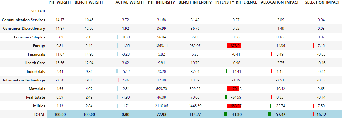
compute_carbon_attribution(portfolio=portfolio_mktcap, grouping='SECTOR', carbon_metric='SCOPE1+2', norm_metric='SALES')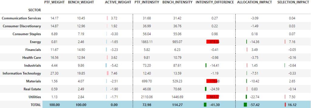
Here with a large cap bias, we are less carbon exposed than the benchmark, mainly due to the UW in Utilities and Energy sectors.
Next use case, we try the analysis on a simple value portfolio (top decile of lower PE values).
# create value portfolio
ptf_assets_value = data.sort_values("PE").head(ptf_nb_assets).index
portfolio_value = data.copy()
portfolio_value.loc[ptf_assets_value, "PTF_WEIGHT"] = portfolio_value["BENCH_WEIGHT"]
portfolio_value.loc[ptf_assets_value, "PTF_WEIGHT"] = portfolio_value.loc[ptf_assets_value, "PTF_WEIGHT"] / portfolio_value.loc[ptf_assets_value, "PTF_WEIGHT"].sum()
portfolio_value["ACTIVE_WEIGHT"] = portfolio_value["PTF_WEIGHT"].fillna(0) - portfolio_value["BENCH_WEIGHT"]

compute_carbon_attribution(portfolio=portfolio_value, grouping='SECTOR', carbon_metric='SCOPE1+2', norm_metric='SALES')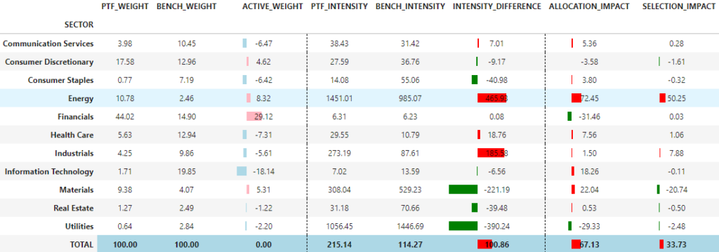
Here we have a higher carbon footprint than the benchmark mainly due to both bad allocation and bad selection effects in the Energy sector.
Finally, same exercise but with a sector neutral value portfolio (best stock decile in each sectors).
# create value sector neutral portfolio
ptf_assets_value_sector_neutral = data.groupby("SECTOR").PE.rank().sort_values().head(ptf_nb_assets).index
portfolio_value_sector_neutral = data.copy()
ranking = data.groupby("SECTOR").apply(lambda x: x["PE"].rank(pct=True, ascending=False)).reset_index()[['level_1',"PE"]]
best_tickers = ranking[ranking["PE"] >= (1-0.1)].level_1 # select top decile for each sector
portfolio_value_sector_neutral['Selected'] = np.where(portfolio_value_sector_neutral.index.isin(best_tickers),1,0)
weighting_scheme = portfolio_value_sector_neutral.groupby("SECTOR").apply(lambda x: (x['BENCH_WEIGHT'] * x['Selected'] / (x['BENCH_WEIGHT'] * x['Selected']).sum()) * x['BENCH_WEIGHT'].sum()).reset_index()[['level_1',0]]
portfolio_value_sector_neutral['PTF_WEIGHT'] = weighting_scheme.set_index('level_1')[0]
portfolio_value_sector_neutral["ACTIVE_WEIGHT"] = portfolio_value_sector_neutral["PTF_WEIGHT"].fillna(0) - portfolio_value_sector_neutral["BENCH_WEIGHT"]

compute_carbon_attribution(portfolio=portfolio_value_sector_neutral, grouping='SECTOR', carbon_metric='SCOPE1+2', norm_metric='SALES')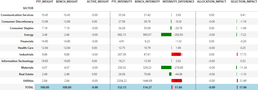
We see in this example that we have indeed neutralized allocation effects, but also improved selection effect!
To conclude, we have shown that different types of portfolio construction techniques can have a big impact on resultant portfolio carbon footprint. With a carbon attribution (here on sectors but could be performed on other groups) we can highlight where are the carbon biases in our portfolio (allocation or selection effect). Not all factor portfolios are equal to carbon exposure. Adding some constraints or neutralization techniques can be useful to reduce carbon emissions while maintaining factor exposure.