Setting up an alpha-generating strategy from scratch: A practical example with a portfolio, made up of equity sectors, investing a simple macro signal
As a quantitative researcher, your main goal is to find new financial edges. In this article, we will show an overview of the pipeline for designing alpha-generating investment strategies, with associated python code as usual.
Here are the main steps that will be presented.
- Investment rationale
- Data collection
- Model training
- Backtesting
- Strategy falsification
- Strategy evaluation
Before starting, an important remark, this article is not made to be completely exhaustive, its main purpose is to share some good practices to the community and not to propose the exact secret recipe of the magic potion. 😉
In the research process, you must first think about the type of relationships you want to exploit. These can relate to company fundamentals, investor behaviors or macroeconomic data to name a few. You find a theme that interests you and strengthen your knowledge by reading existing literature, learning all underlying mechanisms.
In this article we will try to create a strategy thanks to a macroeconomic variable, the US Consumer Price Index (CPI), which is one of the main indicators used to measure US inflation. We act as an equity portfolio manager, who wants to add alpha to its fund through better sector allocation.
Our investment rationale is simple. We have observed that in periods of high or low inflation, equities have dispersed performance. For example, when the price of oil rises, energy stocks tend to benefit. We feel that the equity sectors are not equal when it comes to inflation levels and trends.
We measure inflation by the CPI growth rate, what we call “CPI Year on Year growth” (CPI YoY). We decide to use a simple signal and manually define 4 inflation regimes, based on the difference between CPI YoY versus its 12M average – and the 12M CPI YoY rate of change.
| Regimes | CPI YoY – CPI YoY 12M average | CPI YoY 12M rate of change | Frequency |
| 1 – Lower than average & Falling | – | – | 42.4% |
| 2 – Lower than average & Rising | – | + | 8.8% |
| 3 – Higher than average & Falling | + | – | 6.3% |
| 4 – Higher than average & Rising | + | + | 42.5% |
To this extent, we will analyze the behavior of equity sectors through time and inflation regimes, in order to generate adequate allocations for each inflation regime. These allocations will simply follow a ranking weighting scheme and will be implemented at the close of the effective CPI release date, which is historically provided by FRED, rather than the official month-end date which would add a forward-looking bias.
Now let’s collect the data we need.
First for CPI data, we will retrieve it from the US Federal Reserve’s Economic Database called FRED.
There are already python libraries that make it easy to request data from this source, but for demonstration purposes, we coded a small class called “FredAPI” to get the data ourselves.
For the equity sector return data, we will use the Fama/French data library. There, you can find data on the well-known FF equity factors but also on equity sectors. As for the FRED API, we coded a small class, called “FFData”, to request data we need. We download the FF-5 Factors daily returns and also the 10-industry daily returns that will represent our equity sectors.
For these data we have access to a long history, since 1920s!
However, for our use case, we will use data from 1949 to 2023.
All these classes are included in a file Utilities.py that can be found at the bottom of this article.
from Utilities import *We create our data objects to request our timeseries.
# get macro data
fred = FredAPI(api_key='your_api_key')
# get CPI historical releases dates
cpi_release_dates = fred.getReleaseDates(release_id=10) # CPI-U
# get CPI published data
cpi_ts = fred.getSerieData(serie_id='CPIAUCNS', start_date='1949-02-28', end_date='9999-12-31', flag_real=True) # CPI-U

# convert & adjust date column that should be end of month
cpi_ts['date_adjusted'] = pd.to_datetime(cpi_ts.date, format="%Y-%m-%d") + pd.offsets.MonthEnd(0)
cpi_ts['realtime_start'] = pd.to_datetime(cpi_ts.realtime_start, format="%Y-%m-%d")

# get factors & industries returns
ff = FFData()
# industries
perf_sectors_raw = ff.getIndustryDailyData(data_source='10_Industry_Portfolios', weighting_scheme='value')
# factors
factors_raw = ff.getFactorDailyData()
Model training step
Now we can prepare our data, i.e. split it in training and testing sets. We have in this extent, write a function “prepare_data” to create, align and correct all our features.
train_data = prepare_data(cpi_ts, perf_sectors_raw, cpi_release_dates, start_date='1949-02-28', end_date='1988-12-31', actual=False)
test_data = prepare_data(cpi_ts, perf_sectors_raw, cpi_release_dates, start_date='1988-12-31', end_date='2023-02-28', actual=True)
We select our testing dataset and create our assets returns and regimes timeseries.
assets = test_data.drop(columns=["Regime", "Regime_code"]) / 100
regimes = test_data[["Regime_code"]]
n_assets = len(assets.T)
We create our model allocation thanks to training dataset. We also create a benchmark allocation on the same dates (equal weight allocation).
# ranking weighting scheme
model_allocation = train_data.groupby('Regime_code').mean(numeric_only=True).rank(axis=1, ascending=True) / np.arange(1, n_assets+1).sum()
# equal weight for benchmark
bench_allocation = model_allocation*0 + 1/len(model_allocation.columns)
Backtesting step
Now we can launch our backtest routine, we created a class “Backtest” for all the backtesting logic. We use our testing dataset. On each release date of the CPI, we check if there is a change in regime, if so we rebalance with a new allocation, otherwise we don’t change anything.
# portfolio backtest
bt = Backtest(data_returns=assets, data_trigger=regimes, data_allocation=model_allocation, start_date="1991-12-31", end_date="2023-02-28")
bt.run()
# benchmark backtest
bt_ref = Backtest(data_returns=assets, data_trigger=regimes, data_allocation=bench_allocation, start_date="1991-12-31", end_date="2023-02-28")
bt_ref.run()
# display annualized statistics
bt.compute_stats(bt_ref)| Return | Volatility | Turnover | Sharpe Ratio (w/o cash) | Beta | Tracking Error | Information Ratio | |
| Portfolio | 12.99% | 17.77% | 1.50 | 0.73 | 1.00 | 2.64% | 0.65 |
| Reference | 11.26% | 17.56% | 0.12 | 0.64 | – | – | – |
This result seems good, for a low frequency strategy. Interesting IR and reasonable portfolio turnover (transaction costs for US equities are very low).
Falsification step
Here we will test some alternative scenarii, i.e. falsify our strategy to prove that we really exploited a real effect rather than just being lucky. One possible way is to invert our regimes periods. Like this.
# falsification 1
regimes_false = (test_data[["Regime_code"]]-2).replace(-1,2).replace(-2,3)
bt_false = Backtest(data_returns=assets, data_trigger=regimes_false, data_allocation=model_allocation, start_date="1991-12-31", end_date="2023-01-31")
bt_false.run()
bt_false.compute_stats(bt_ref)

# falsification 2
regimes_false2 = (test_data[["Regime_code"]]-1).replace(-1,3)
bt_false2 = Backtest(data_returns=assets, data_trigger=regimes_false2, data_allocation=model_allocation, start_date="1991-12-31", end_date="2023-01-31")
bt_false2.run()
bt_false2.compute_stats(bt_ref)

# falsification 3
regimes_false3 = np.abs(test_data[["Regime_code"]]-3)
bt_false3 = Backtest(data_returns=assets, data_trigger=regimes_false3, data_allocation=model_allocation, start_date="1991-12-31", end_date="2023-01-31")
bt_false3.run()
bt_false3.compute_stats(bt_ref)| Return | Volatility | Turnover | Sharpe Ratio (w/o cash) | Beta | Tracking Error | Information Ratio | |
| Falsification #1 | 10.81% | 17.73% | 1.62 | 0.61 | 1.00 | 2.44% | -0.18 |
| Falsification #2 | 10.41% | 17.31% | 1.50 | 0.60 | 0.98 | 2.32% | -0.36 |
| Falsification #3 | 9.46% | 17.73% | 1.49 | 0.53 | 0.99 | 3.02% | -0.59 |
If our hypothesis was false, or at least had no impact on performance, we should have the same results on all backtests regardless of the inflation regime set.
Strategy evaluation step
Now that we confirmed that we have a real edge, we can assess if our strategy produces alpha versus our benchmark and the market.
# against reference benchmark
X = bt_ref.portfolio_perf.Perf.dropna()
y = bt.portfolio_perf.Perf.dropna()
model = sm.GLS(y,sm.add_constant(X))
res = model.fit()
res.summary()
print(res.params[0]*260) # annualized alpha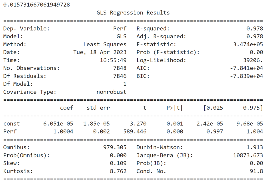
We have a beta (vs reference) close to 1 and a positive annualized alpha of 1.57%, the loadings are statistically robust.
We can do the same exercise, but with the FF-5 Factors instead of our reference strategy.
# against FF-5 factors
y = bt.portfolio_perf.Perf.dropna()
X = factors_raw.drop(columns=['RF']) / 100
X = X.loc[y.index]
y = y.loc[X.index]
model = sm.GLS(y,sm.add_constant(X))
res = model.fit()
res.summary()
print(res.params.const*260) # annualized alpha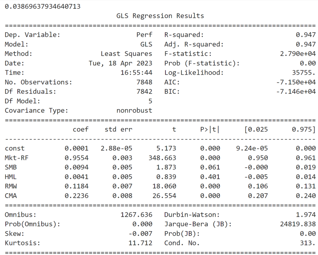
With this model, we have a low market beta of 0.95, neutral exposure to Size (SMB) and Value (HML), positive exposure to Profitability (RMW) and Investment (CMA). The alpha is robust and positive, around 3.8% annually.
We may also check, on a rolling window, market beta and alpha behaviors.
# we can also check the stability of alpha and market beta coefficients through time
model_roll = RollingOLS(y, sm.add_constant(X), window=260)
res_roll = model_roll.fit()
plt.figure(figsize=(10, 6))
(res_roll.params.const*260).plot()
(res_roll.params.const*0+res_roll.params.const.mean()*260).plot(linestyle='dashed')
plt.figure(figsize=(10, 6))
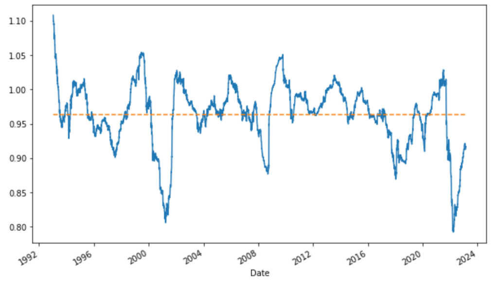
(res_roll.params['Mkt-RF']).plot()
(res_roll.params['Mkt-RF']*0+res_roll.params['Mkt-RF'].mean()).plot(linestyle='dashed')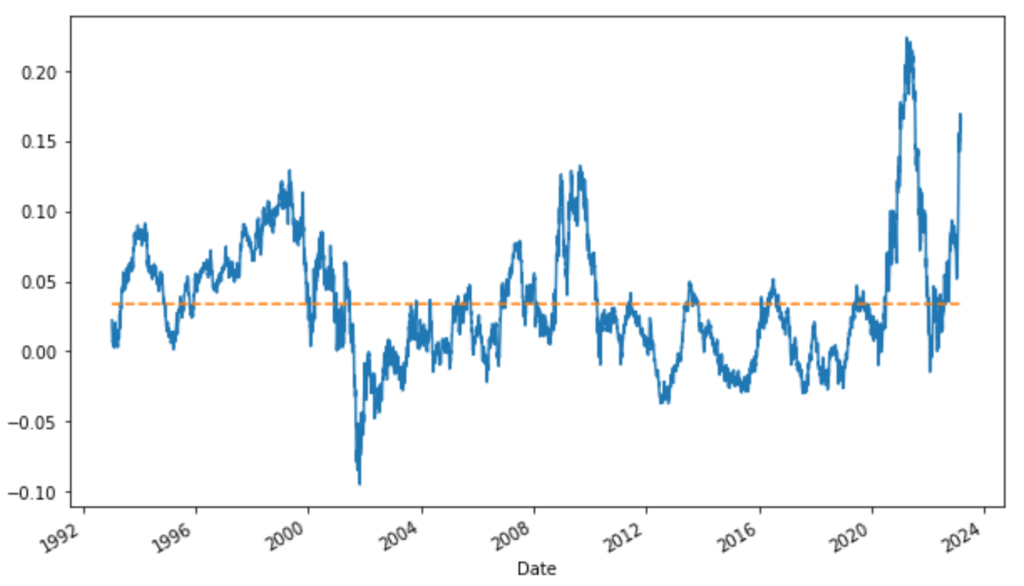
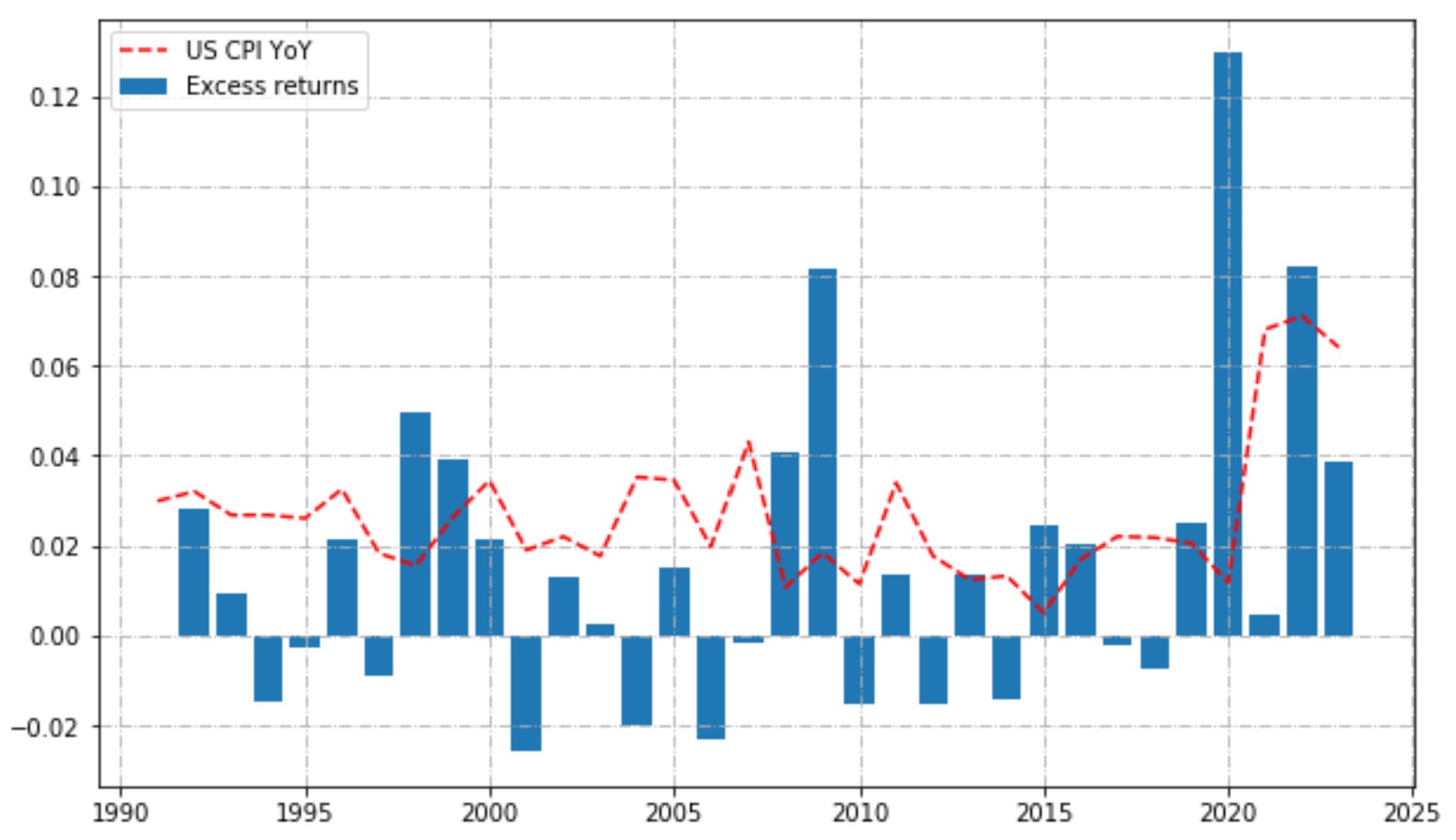
We can have a look at annual calendar performances, to see if returns were stable over time.
# calendar returns
calendar_returns = pd.concat([(bt.portfolio_perf.Value.groupby(bt.portfolio_perf.index.year).last() / bt.portfolio_perf.Value.groupby(bt.portfolio_perf.index.year).last().shift(1) - 1),
          bt_ref.portfolio_perf.Value.groupby(bt_ref.portfolio_perf.index.year).last() / bt_ref.portfolio_perf.Value.groupby(bt_ref.portfolio_perf.index.year).last().shift(1) - 1], axis=1, ignore_index=True).transpose().dropna(axis=1).rename(index={0:'Ptf', 1:'Ref'}).transpose()
calendar_returns["Excess"] = calendar_returns["Ptf"] - calendar_returns["Ref"]
plt.figure(figsize=(10, 6))
plt.plot(test_data.value_yoy.resample('Y').last().index.year, test_data.value_yoy.resample('Y').last(),
linestyle="dashed", alpha=2, label="US CPI YoY", color='red')
plt.bar(calendar_returns.index, calendar_returns.Excess, label='Excess returns')
plt.legend()
plt.grid(True, linestyle="-.")
plt.show()
We can also have a look at the return distribution of our strategy.
moments = pd.DataFrame(index=["Ann. Mean","Ann. Variance","Skewness","Kurtosis"], columns=calendar_returns.columns)
moments.loc["Ann. Mean", "Ptf"] = bt.portfolio_perf.Perf.mean() * 260
moments.loc["Ann. Variance", "Ptf"] = bt.portfolio_perf.Perf.var() * 260
moments.loc["Skewness", "Ptf"] = bt.portfolio_perf.Perf.skew()
moments.loc["Kurtosis", "Ptf"] = bt.portfolio_perf.Perf.kurt()

moments.loc["Ann. Mean", "Ref"] = bt_ref.portfolio_perf.Perf.mean() * 260
moments.loc["Ann. Variance", "Ref"] = bt_ref.portfolio_perf.Perf.var() * 260
moments.loc["Skewness", "Ref"] = bt_ref.portfolio_perf.Perf.skew()
moments.loc["Kurtosis", "Ref"] = bt_ref.portfolio_perf.Perf.kurt()

moments.loc["Ann. Mean", "Excess"] = (bt.portfolio_perf.Perf - bt_ref.portfolio_perf.Perf).mean() * 260
moments.loc["Ann. Variance", "Excess"] = (bt.portfolio_perf.Perf - bt_ref.portfolio_perf.Perf).var() * 260
moments.loc["Skewness", "Excess"] = (bt.portfolio_perf.Perf - bt_ref.portfolio_perf.Perf).skew()
moments.loc["Kurtosis", "Excess"] = (bt.portfolio_perf.Perf - bt_ref.portfolio_perf.Perf).kurt()| Ptf | Ref | Excess | |
| Ann. Mean | 0.137955 | 0.122172 | 0.0157832 |
| Ann. Variance | 0.0315724 | 0.0308491 | 0.000697226 |
| Skewness | -0.215768 | -0.297998 | 0.109316 |
| Kurtosis | 11.6345 | 11.4875 | 5.77481 |
Through the estimation of the moments of the excess return distribution of the strategy, we assessed that we have a higher mean at the cost of higher variance and higher kurtosis (higher tail risk). However our strategy (excess) is positively skewed which means that extreme events tend to be on the positive side (frequent small losses and few large gains).
From all these results, the portfolio manager finds that this strategy could be a good diversifier of his overall strategy and chooses to give it some budget in his tactical pocket!
To conclude, in this article we presented an overview of the main steps in designing alpha-generating strategies. Start by seriously thinking about the rationale of your strategy, then collect and adjust your data. Leverage data efficiently with separate training and testing sets to create a robust investment model. Back-test your results across multiple market regimes and most importantly falsify your strategy to assess the validity of the strategy. Finally check if you have produced significant and stable alpha over time while also checking your returns distribution profile.
Annex
Below are all utility classes and functions used in this article.
import pandas as pd
import numpy as np
import requests
import matplotlib.pyplot as plt
from tqdm import tqdm
import statsmodels.api as sm
from statsmodels.regression.rolling import RollingOLS
from zipfile import ZipFile
import tempfile
from io import StringIO
from urllib3.exceptions import InsecureRequestWarning
from urllib3 import disable_warnings

disable_warnings(InsecureRequestWarning)

class FFData():
    """A set of methods to get financial data from the FF data library"""
    def __init__(self):
        """Create the request object"""
        self.s = requests.Session()
        self.baseURL = "https://mba.tuck.dartmouth.edu/pages/faculty/ken.french/"

    def getFactorDailyData(self):
        """ Get 5-factor data from a specific Fama French data source """
        downloadURL = self.baseURL + 'ftp/F-F_Research_Data_5_Factors_2x3_daily_CSV.zip'
        download = self.s.get(url=downloadURL, verify=False)

        with tempfile.TemporaryFile() as tmpf:
            tmpf.write(download.content)
            with ZipFile(tmpf, "r") as zf:
                data = zf.open(zf.namelist()[0]).read().decode()
        df = pd.read_csv(StringIO(data), engine='python', skiprows=3, skipfooter=0, decimal='.', sep=',').rename(columns={'Unnamed: 0':'Date'})
        df_filtered = df.copy()
        df_filtered.Date = pd.to_datetime(df_filtered.Date, format="%Y%m%d")
        df_filtered = df_filtered.set_index("Date")
        return df_filtered.astype(float)

    def getIndustryDailyData(self, data_source='10_Industry_Portfolios', weighting_scheme='value'):
        """ Get industry data from a specific Fama French data source """
        downloadURL = self.baseURL + 'ftp/%s_daily_CSV.zip'%(data_source)
        download = self.s.get(url=downloadURL, verify=False)

        with tempfile.TemporaryFile() as tmpf:
            tmpf.write(download.content)
            with ZipFile(tmpf, "r") as zf:
                data = zf.open(zf.namelist()[0]).read().decode()
        df = pd.read_csv(StringIO(data), engine='python', skiprows=9, skipfooter=1, decimal='.', sep=',').rename(columns={'Unnamed: 0':'Date'})
        if weighting_scheme == 'value':
            keep_flag = 'first' # keep value weighted returns
        else:
            keep_flag = 'last' # keep equal weighted returns
        df_filtered = df.loc[df[df.Date.str.isnumeric() == True].drop_duplicates(subset=['Date'], keep=keep_flag).index]
        df_filtered.Date = pd.to_datetime(df_filtered.Date, format="%Y%m%d")
        df_filtered = df_filtered.set_index("Date")
        return df_filtered.astype(float)

class FredAPI():
    """A set of methods to get economic data from the FRED® and ALFRED® websites hosted by the Economic Research Division of the Federal Reserve Bank of St. Louis. Requests can be customized according to data source, release, category, series, and other preferences."""
    def __init__(self, api_key):
        """Create the request object"""
        self.s = requests.Session()
        self.api_key = api_key
        self.baseURL = "https://api.stlouisfed.org/fred/"

    def getAllReleases(self):
        """ Get all available releases """
        downloadURL = self.baseURL + 'releases?api_key=%s&file_type=json'%(self.api_key)
        download = self.s.get(url=downloadURL)
        return pd.DataFrame(download.json()['releases'])

    def getReleaseDates(self, release_id=10):
        """ Get release dates for a specific economic variable """
        downloadURL = self.baseURL + '/release/dates?release_id=%s&api_key=%s&file_type=json'%(release_id, self.api_key)
        download = self.s.get(url=downloadURL)
        return pd.DataFrame(download.json()['release_dates'])

    def getReleaseLinkedSeries(self, release_id=10):
        """ Get economic series for a specific release of economic data"""
        downloadURL = self.baseURL + '/release/series?release_id=%s&api_key=%s&file_type=json'%(release_id, self.api_key)
        download = self.s.get(url=downloadURL)
        return pd.DataFrame(download.json()['seriess'])

    def getSerieData(self, serie_id='CPIAUCNS', start_date='', end_date='', flag_real=False):
        """ Get observations time serie for a specific economic variable """
        if flag_real == True:
            downloadURL = self.baseURL + '/series/observations?series_id=%s&api_key=%s&observation_start=%s&observation_end=%s&realtime_start=%s&realtime_end=%s&file_type=json'%(serie_id, self.api_key, start_date, end_date, start_date, end_date)
        else:
            downloadURL = self.baseURL + '/series/observations?series_id=%s&api_key=%s&observation_start=%s&observation_end=%s&file_type=json'%(serie_id, self.api_key, start_date, end_date)
        download = self.s.get(url=downloadURL)
        df = pd.DataFrame(download.json()['observations'])
        df["value"] = pd.to_numeric(df["value"])
        return df

class Backtest():
    """ A set of methods to backtest a 10-industry portfolio following a regime portfolio allocation model  """
    def __init__(self, data_returns, data_trigger, data_allocation, start_date="1951-03-31", end_date="1989-12-31"):
        # convert to datetime
        self.start_date = pd.to_datetime(start_date, format='%Y-%m-%d')
        self.end_date = pd.to_datetime(end_date, format='%Y-%m-%d')
        # subsample data accordingly
        self.returns = data_returns.loc[self.start_date:self.end_date]
        self.trigger = data_trigger.loc[self.start_date:self.end_date]
        self.allocation_model = data_allocation
        self.portfolio = pd.DataFrame(index=self.returns.index, columns=self.returns.columns)
        self.portfolio_perf = pd.DataFrame(index=self.returns.index, columns=["Value", "Perf", "Turnover"], dtype=float)
        # initiate portfolio composition
        self.current_state = -1
        self.current_portfolio = 1/len(self.allocation_model.columns)
        self.portfolio.loc[self.start_date] = self.current_portfolio
        self.current_value = 100
        self.portfolio_perf.loc[self.start_date, "Value"] = self.current_value
        # start after first period
        self.dates_to_run = self.returns.iloc[1:].index

    def _event(self, dt):
        # check if there is a new state, return 1 if yes, else 0
        self.new_state = self.trigger.loc[dt].values[0]
        if self.new_state != self.current_state:
            return 1
        else:
            return 0

    def _rebalance(self, dt):
        # apply allocation model
        previous_ptf = self.current_portfolio
        current_returns = self.returns.loc[dt]
        new_ptf = self.allocation_model.loc[self.new_state]
        previous_ptf_drifted = previous_ptf * (1 + current_returns)
        # compute new nav and performance
        self.portfolio_perf.loc[dt, "Value"] = self.current_value * previous_ptf_drifted.sum()
        self.portfolio_perf.loc[dt, "Perf"] = (current_returns * previous_ptf).sum()
        # also compute turnover of end-of-period weights versus new weights
        self.portfolio_perf.loc[dt, "Turnover"] = np.sum(np.abs(new_ptf - (previous_ptf_drifted / previous_ptf_drifted.sum())))
        # save new weights from alloc model
        self.portfolio.loc[dt] = new_ptf

    def _drift(self, dt):
        # compute drifted weights
        previous_ptf = self.current_portfolio
        current_returns = self.returns.loc[dt]
        previous_ptf_drifted = previous_ptf * (1 + current_returns)
        new_ptf = previous_ptf_drifted / previous_ptf_drifted.sum()
        # compute new nav and performance
        self.portfolio_perf.loc[dt, "Value"] = self.current_value * previous_ptf_drifted.sum()
        self.portfolio_perf.loc[dt, "Perf"] = (current_returns * previous_ptf).sum()
        self.portfolio_perf.loc[dt, "Turnover"] = np.nan # no turnover
        # save drifted weights
        self.portfolio.loc[dt] = new_ptf
        return 0

    def compute_stats(self, reference=None):
        # compute statistic analysis of the backtest
        stats = pd.DataFrame(index=["Portfolio", "Benchmark"], columns=["Return", "Volatility", "Turnover"], dtype=float)
        stats.loc["Portfolio", "Return"] = self.portfolio_perf.Perf.add(1).prod() ** (260 / len(self.portfolio_perf)) - 1
        stats.loc["Portfolio", "Volatility"] = self.portfolio_perf.Perf.std() * np.sqrt(260)
        stats.loc["Portfolio", "Sharpe Ratio"] = stats.loc["Portfolio", "Return"] / stats.loc["Portfolio", "Volatility"]
        stats.loc["Portfolio", "Turnover"] = self.portfolio_perf.groupby(self.portfolio_perf.index.year).sum().Turnover.mean()
        if reference is not None:
            stats.loc["Benchmark", "Return"] = reference.portfolio_perf.Perf.add(1).prod() ** (260 / len(reference.portfolio_perf)) - 1
            stats.loc["Benchmark", "Volatility"] = reference.portfolio_perf.Perf.std() * np.sqrt(260)
            stats.loc["Benchmark", "Sharpe Ratio"] = stats.loc["Benchmark", "Return"] / stats.loc["Benchmark", "Volatility"]
            stats.loc["Benchmark", "Turnover"] = reference.portfolio_perf.groupby(reference.portfolio_perf.index.year).sum().Turnover.mean()
            stats.loc["Portfolio", "Beta"] = pd.concat([self.portfolio_perf.Perf,reference.portfolio_perf.Perf],axis=1).cov().iloc[0,1] / reference.portfolio_perf.Perf.var()
            stats.loc["Portfolio", "Tracking Error"] = (self.portfolio_perf.Perf-reference.portfolio_perf.Perf).std() * np.sqrt(260)
            stats.loc["Portfolio", "Information Ratio"] = (stats.loc["Portfolio", "Return"] - stats.loc["Benchmark", "Return"]) / stats.loc["Portfolio", "Tracking Error"]
        return stats

    def run(self):
        for dt in tqdm(self.dates_to_run):
            if self._event(dt) == 1:
                self._rebalance(dt)
            else:
                self._drift(dt)
            self.current_state = self.new_state # assign new state
            self.current_value = self.portfolio_perf.loc[dt, "Value"] # assign new nav
            self.current_portfolio = self.portfolio.loc[dt] # assign new portfolio


def prepare_data(data_signal, data_returns, cpi_releases, start_date='1988-12-31', end_date='2023-01-31', actual=True):
    """ A function to create inflation features and choose the release date, i.e. actual or end of month """
    if actual == True:
        cpi_releases["real_date"] = pd.to_datetime(cpi_releases.date, format="%Y-%m-%d")
        mapping = cpi_releases.merge(data_signal.sort_values('realtime_start').drop_duplicates(subset='date_adjusted', keep='first').sort_values('date_adjusted')[["realtime_start", "date_adjusted"]], how='left', right_on='realtime_start', left_on='real_date')[["date_adjusted", "real_date"]].dropna()
        signal = data_signal.sort_values('realtime_start').drop_duplicates(subset='date_adjusted', keep='last').sort_values('date_adjusted')[["date_adjusted", "value"]].merge(mapping, how='left', on='date_adjusted')
    else:
        signal = data_signal.sort_values('realtime_start').drop_duplicates(subset='date_adjusted', keep='last').sort_values('date_adjusted')
    signal = signal.loc[(signal.date_adjusted >= start_date) & (signal.date_adjusted <= end_date)]
    signal['value_yoy'] = signal.value / signal.value.shift(12) - 1
    signal['value_yoy_mean'] = signal['value_yoy'].rolling(12).mean() # mean inflation rate of last 12M
    signal['value_yoy_rate'] = signal['value_yoy'] - signal['value_yoy'].shift(12) # rate of change of inflation

    conditionList = [(signal['value_yoy'] < signal['value_yoy_mean']) & (signal['value_yoy_rate'] < 0),
                     (signal['value_yoy'] < signal['value_yoy_mean']) & (signal['value_yoy_rate'] >= 0),
                     (signal['value_yoy'] >= signal['value_yoy_mean']) & (signal['value_yoy_rate'] < 0),
                     (signal['value_yoy'] >= signal['value_yoy_mean']) & (signal['value_yoy_rate'] >= 0)]
    choiceList = ['Lower & Falling', 'Lower & Rising', 'Higher & Falling', 'Higher & Rising']
    choiceList_code = [0, 1, 2, 3]
    signal['Regime'] = np.select(conditionList, choiceList, default=np.nan)
    signal['Regime_code'] = np.select(conditionList, choiceList_code, default=np.nan)
    signal.dropna(inplace=True)
    data_returns = data_returns.loc[(data_returns.index >= start_date) & (data_returns.index <= end_date)]
    if actual == True:
        prepared_data = data_returns.merge(signal[['real_date','Regime','Regime_code']] \
                                                  .set_index('real_date'), how='left', right_index=True, left_index=True) \
                                                  .fillna(method="ffill").dropna()
    else:
        prepared_data = data_returns.merge(signal[['date_adjusted','Regime','Regime_code']] \
                                                  .set_index('date_adjusted'), how='left', right_index=True, left_index=True) \
                                                  .fillna(method="ffill").dropna()
    return prepared_data