Protected equity fund: Split your portfolio to better fit your hedging instruments.
Imagine you are an European insurer. One of your funds is an equity portfolio of EMU stocks. Under Solvency II framework, you might want to reduce your Solvency Capital Requirement (SCR) thanks to the use of derivatives to hedge some of your equity risk. However, due to your size, the only sufficiently liquid contracts that you can use are Euro Stoxx 50 (E50) options. The problem is that your fund invest in a wider stock universe and the tracking error of your fund versus E50 index is quite high. This means that you will have non negligible basis risk in your hedge, which could be a lot more material in case of stressed markets.
One solution would be to “sort” your portfolio, i.e. split it into a core pocket (that we will hedge) and a residual pocket. The core pocket being the portfolio containing the best mix of stocks to reduce the active risk compared to the E50 index (our reference benchmark), the remaining inventory being mapped onto a residual portfolio.
How much stock can we add to the core pocket while seeking to improve its tracking error relative to the benchmark?
There are two ways to solve this trade-off issue, one is to map a maximum number of stocks to the core portfolio under an active risk constraint below a specified threshold, the other one is to define the level of hedge you want to apply and find the best core pocket covering this hedge ratio.
The optimization
The objective is to find the minimum tracking error sub-portfolio inside our portfolio, taking the hypothesis of a core portfolio size target.
This can be written as the following convex problem.
w^*\ =\argmin\ \{  \ w_{rel}^\top \Sigma\ w_{rel}  \}\\
\newline\
\\
w.r.t:  \begin{cases} \sum w = 1 \\
A_{core}\ \cdot\ w \leq MV_{max}
\end{cases}
\newline\
\\
with\  \begin{cases} \Sigma\ :\ covariance\ matrix \\
w_{rel} = w - w_{bench} \\
w_{bench}\ :\ weight\ of\ stocks\ in\ reference\ benchmark \\
A_{core}\ :\ target\ core\ portfolio\ size \\
MV_{max} =\ p\ \cdot\ h \Leftrightarrow\ stocks\ market\ value\ in\ total\ portfolio \\
p\ :\ stocks\ prices\ \\
h\ :\ number\ of\ shares\ held\ in\ total\ portfolio \\
\end{cases}
Practical example
We have a portfolio worth of €1B, invested on 80 EMU stocks, and we would like to hedge it with E50 options. We would like to show the cost of hedging (in term of basis risk) on several portions of the portfolio, to determine how much of the €1B we are willing to hedge.
Now let’s code it!
import pandas as pd
import numpy as np
import cvxpy as cvx
We define our inputs and parameters. Let’s start with a target core portfolio of €500M.
# we load our portfolio
portfolio = pd.DataFrame(columns=['Asset Name', 'Price', 'Holdings', 'Bmk Weight (%)'])
# assets' market value in portfolio
portfolio['Market Value'] = portfolio['Price'] * portfolio['Holdings']
# assets' weights in portfolio
portfolio['Weight Ptf (%)'] = portfolio['Market Value'] / portfolio['Market Value'].sum()

# number of stocks in universe
n = len(portfolio)
# our target core portfolio size
core_aum = 50e7
# maximum market value for each asset
mv_max = portfolio['Market Value'].values
# assets' weight in benchmark
w_bench = portfolio['Bmk Weight (%)'].values
# optimal core weights to find
w = cvx.Variable(n, pos=True)
We write down our problem and solve it.
constraints = [cvx.sum(w) == 1, w * core_aum <= mv_max]
utility = cvx.quad_form(w-w_bench, Sigma) # Sigma is our covariance matrix
objective = cvx.Minimize(utility)
prob = cvx.Problem(objective, constraints)
prob.solve(verbose=False, solver='XPRESS')
From the optimization results, we find the number of holdings (integer) and adjust stocks core weights and market values accordingly.
# Store raw results
portfolio['Raw Weight Core (%)'] = w.value

# convert to raw MV
portfolio['Raw Market Value Core'] = portfolio['Raw Weight Core (%)'] * core_aum

# find the actual number of holdings (integer)
portfolio['Holding Core'] = np.floor(portfolio['Raw Market Value Core'] / portfolio['Price'])

# compute the effective MV
portfolio['Market Value Core'] = portfolio['Holding Core'] * portfolio['Price']

# compute the effective weight
portfolio['Weight Core (%)'] = portfolio['Market Value Core'] / portfolio['Market Value Core'].sum()

# compute raw core tracking error
raw_active_risk_core = np.sqrt((portfolio['Raw Weight Core (%)'] - portfolio['Bmk Weight (%)'].values) @ Sigma @ (portfolio['Raw Weight Core (%)'].values - portfolio['Bmk Weight (%)'].values))

# compute core tracking error
active_risk_core = np.sqrt((portfolio['Weight Core (%)'] - portfolio['Bmk Weight (%)'].values) @ Sigma @ (portfolio['Weight Core (%)'].values - portfolio['Bmk Weight (%)'].values))

# compute total portfolio tracking error
active_risk_ptf = np.sqrt((portfolio['Weight Ptf (%)'] - portfolio['Bmk Weight (%)'].values) @ Sigma @ (portfolio['Weight Ptf (%)'].values - portfolio['Bmk Weight (%)'].values))
We now have the following results.
print(raw_active_risk_core)
# 2.90%
print(active_risk_core)
# 2.90%
print(active_risk_ptf)
# 4.00%
We see that there is no impact on the tracking error between the raw and adjusted core portfolio, as equity lot sizes are quite small. We have quite improved our active risk compared to the total portfolio which has a tracking error of 4%.
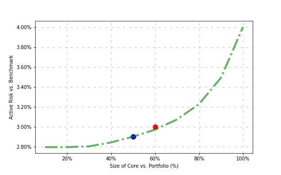
Now let’s see for several core portfolio sizes how does the tracking error level reacts.
From these results, we can now decide what to do.
- If our objective was to find the largest core portfolio with a maximum tracking error level of 3%, we can have a sub-portfolio size up to ~€600M.
- Or if our objective was to hedge let’s say 50% of our portfolio, taking the associated core portfolio we have reduced our basis risk of nearly 28%, lowering the active risk from 4% to 2.9%.