Replicate Fama French 5-Factor Model from publicly available data sources
As an equity quantitative analyst, you have recurring positioning analysis tasks. Your most effective approach is to model your object of study (usually stocks, portfolios or indexes) and decompose its behavior into common risk factors. You can create your own “factor model” or use existing models. There are robust models generated by data providers like MSCI or Qontigo, which are quite expensive but necessary for large institutions. Otherwise you have lighter academic models like the famous five-factor model developed by Fama-French.
In this article, we will try to reproduce the last one.
The FF-5 model is freely available but it is published with a 2 month lag, which is why it is interesting to create a proxy to recover these missing months, in order to produce a live analysis.
One difficulty that immediately arises is the sourcing of data. Academic research often use CRSP database. But it is reserved for academic practitioners and not free. We can wonder if we can reproduce, or at least have very close results, with publicly available data. For that, we will leverage the python library yfinance which interacts with Yahoo Finance APIs to download all the financial data we will need.
For the automatic download of Fama French original data, please refer to this previous article.
import pandas as pd
import numpy as np
import yfinance as yf
import requests
from tqdm import tqdm
import statsmodels.api as sm
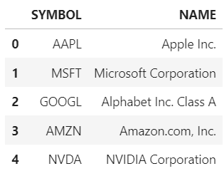
We start with a list containing around 2500 tickers of US stocks (~99% of US market cap).
ticker_list.head()
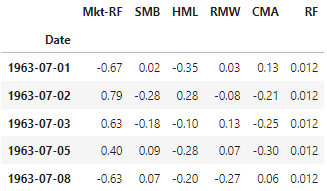
We load Fama French factor returns, these are the timeseries that we will try to replicate.
data_ff.head()
We have to specify a few dates to request the data. Following Fama French website methodology, portfolios are made each year at the end of June, with most recent fundamental data available at the end of last calendar year. Here we create the June 2023 baskets, to assess replication from July 2023 to maximum June 2024. Last calendar year is 2022.
start_date = "2021-12-31"
end_date = "2024-03-29"
start_year_y1 = "2022-01-01"
end_year_y1 = "2022-12-30"
cutoff_year = "2022-12"
cutoff_date = "2023-06-30"
cutoff_date_y1 = "2022-06-30"
last_ff_date = "2024-01-31"

risk_free_rate = data_ff.RF.iloc[-1] # we take the last available risk free rate number
We request, from yahoo api, the following metrics: operating income (or net income if missing), total assets, stockholder’s equity, number of shares and shares close prices.
operating_income = pd.DataFrame() # needed for RMW
total_assets = pd.DataFrame() # needed for CMA
book_value = pd.DataFrame() # needed for HML
nb_shares = pd.DataFrame(index=pd.date_range(start_year_y1, cutoff_date, freq="D")) # number of stock's shares
share_price = pd.DataFrame() # prices

s = requests.Session()

for this_ticker in tqdm(ticker_list.SYMBOL):
    stock = yf.Ticker(this_ticker, session=s)
    if stock.financials.empty: # check if ticker exists, otherwise skip stock
        continue
    # operating income
    try: # standard formula
        if operating_income.empty:
            operating_income = stock.financials.loc["Operating Income"].rename(this_ticker)
        else:
            operating_income = pd.concat([operating_income, stock.financials.loc["Operating Income"].rename(this_ticker)], axis=1)
    except:
        try: # if operating income metric is missing, we take net income
            if operating_income.empty:
                operating_income = (stock.financials.loc['Net Income']).rename(this_ticker)
            else:
                operating_income = pd.concat([operating_income, (stock.financials.loc['Net Income']).rename(this_ticker)], axis=1)
        except: # otherwise skip this stock
            continue
    # total asset
    if total_assets.empty:
        total_assets = stock.balance_sheet.loc["Total Assets"].rename(this_ticker)
    else:
        total_assets = pd.concat([total_assets, stock.balance_sheet.loc["Total Assets"].rename(this_ticker)], axis=1)
    # book value
    if book_value.empty:
        book_value = stock.balance_sheet.loc["Stockholders Equity"].rename(this_ticker)
    else:
        book_value = pd.concat([book_value, stock.balance_sheet.loc["Stockholders Equity"].rename(this_ticker)], axis=1)
    # number of shares
    try: #first method
        nb_shares_new = stock.get_shares_full(start=start_year_y1, end=cutoff_date).rename(this_ticker).drop_duplicates().tz_localize(None)
        nb_shares.loc[nb_shares_new.index, this_ticker] = nb_shares_new
    except: # if no data, test second method
        nb_shares_new = stock.balance_sheet.loc["Ordinary Shares Number"].rename(this_ticker)
        nb_shares.loc[:, this_ticker] = nb_shares_new.loc[nb_shares_new.index.isin(nb_shares.index)]
    # price of share
    if share_price.empty:
        share_price = stock.history(start=start_date, end=end_date).Close.rename(this_ticker)
    else:
        share_price = pd.concat([share_price, stock.history(start=start_date, end=end_date).Close.rename(this_ticker)], axis=1)
share_price.index = pd.to_datetime(share_price.index.strftime("%Y%m%d"))
share_return = (share_price / share_price.shift(1) - 1).fillna(0) # compute price returns
Now with the downloaded raw data, we can compute the fundamental metrics & ratios.
factor_metric = pd.DataFrame(index=ticker_list.SYMBOL, columns=["HML", "SMB", "RMW", "CMA"], dtype="float")
# SMB: price x nb shares = market cap
market_cap = share_price.loc[cutoff_date] * nb_shares.infer_objects().ffill().loc[cutoff_date]
factor_metric.loc[market_cap.index, "SMB"] = market_cap
# HML: book to market ratio
book_market = book_value.infer_objects().ffill().loc[cutoff_year] / (share_price.loc[end_year_y1] * nb_shares.infer_objects().ffill().loc[end_year_y1])
factor_metric.loc[book_market.columns, "HML"] = book_market.values
# RMW: operating income / book value
operating_profit = operating_income.infer_objects().ffill().loc[cutoff_year] / book_value.infer_objects().ffill().loc[cutoff_year]
factor_metric.loc[operating_profit.columns, "RMW"] = operating_profit.values
# CMA: total asset 1Y growth
investment = total_assets.infer_objects().ffill().loc[cutoff_date] / total_assets.infer_objects().ffill().loc[cutoff_date_y1] - 1
factor_metric.loc[investment.index, "CMA"] = investment
We filter the investment universe to keep only stocks that have positive book to market ratios. We compute metrics thresholds to map stocks into the long and short legs.
filtered_metric = factor_metric[factor_metric.HML > 0].copy()

# Define thresholds
mktcap_threshold = filtered_metric.SMB.quantile(0.5)

high_threshold =  filtered_metric.HML.quantile(0.7)
low_threshold =  filtered_metric.HML.quantile(0.3)

robust_threshold =  filtered_metric.RMW.quantile(0.7)
weak_threshold =  filtered_metric.RMW.quantile(0.3)

aggress_threshold =  filtered_metric.CMA.quantile(0.7)
conserv_threshold =  filtered_metric.CMA.quantile(0.3)
We create 4 baskets for each factor (HML, RMW, CMA). No need for SMB, as it is a combination of these.
basket_compo = filtered_metric.copy().drop(columns=["SMB"])
# HML
basket_compo['HML'] = None
basket_compo['HML'] = basket_compo['HML'].astype(str)
basket_compo.loc[(filtered_metric.SMB < mktcap_threshold) & (filtered_metric.HML >= high_threshold), "HML"] = "small_high"
basket_compo.loc[(filtered_metric.SMB < mktcap_threshold) & (filtered_metric.HML <= low_threshold), "HML"] = "small_low"
basket_compo.loc[(filtered_metric.SMB >= mktcap_threshold) & (filtered_metric.HML >= high_threshold), "HML"] = "big_high"
basket_compo.loc[(filtered_metric.SMB >= mktcap_threshold) & (filtered_metric.HML <= low_threshold), "HML"] = "big_low"
# RMW
basket_compo['RMW'] = None
basket_compo['RMW'] = basket_compo['RMW'].astype(str)
basket_compo.loc[(filtered_metric.SMB < mktcap_threshold) & (filtered_metric.RMW >= robust_threshold), "RMW"] = "small_robust"
basket_compo.loc[(filtered_metric.SMB < mktcap_threshold) & (filtered_metric.RMW <= weak_threshold), "RMW"] = "small_weak"
basket_compo.loc[(filtered_metric.SMB >= mktcap_threshold) & (filtered_metric.RMW >= robust_threshold), "RMW"] = "big_robust"
basket_compo.loc[(filtered_metric.SMB >= mktcap_threshold) & (filtered_metric.RMW <= weak_threshold), "RMW"] = "big_weak"
# CMA
basket_compo['CMA'] = None
basket_compo['CMA'] = basket_compo['CMA'].astype(str)
basket_compo.loc[(filtered_metric.SMB < mktcap_threshold) & (filtered_metric.CMA >= aggress_threshold), "CMA"] = "small_aggress"
basket_compo.loc[(filtered_metric.SMB < mktcap_threshold) & (filtered_metric.CMA <= conserv_threshold), "CMA"] = "small_conserv"
basket_compo.loc[(filtered_metric.SMB >= mktcap_threshold) & (filtered_metric.CMA >= aggress_threshold), "CMA"] = "big_aggress"
basket_compo.loc[(filtered_metric.SMB >= mktcap_threshold) & (filtered_metric.CMA <= conserv_threshold), "CMA"] = "big_conserv"
We have all the data needed to compute returns for long and short baskets for each factor. In the FF methodology factors are composed in June and weights are kept constant every day until June Y+1.
basket_weight = filtered_metric.copy().drop(columns=["SMB"])
basket_hml = pd.DataFrame(index=share_return.index, columns=["small_high", "small_low", "big_high", "big_low"])
basket_rmw = pd.DataFrame(index=share_return.index, columns=["small_robust", "small_weak", "big_robust", "big_weak"])
basket_cma = pd.DataFrame(index=share_return.index, columns=["small_aggress", "small_conserv", "big_aggress", "big_conserv"])

# HML
basket_weight["HML"] = np.nan
for bskt in basket_hml.columns:
  	# compute weight, which is market cap weighted
    basket_weight.loc[basket_compo.HML == bskt, "HML"] = filtered_metric[basket_compo.HML == bskt].SMB / filtered_metric[basket_compo.HML == bskt].SMB.sum()
    ret = share_return.loc[:, basket_compo[basket_compo.HML == bskt].index] # get returns of selected stocks
    wgt = basket_weight[basket_compo.HML == bskt].HML.values # get weighting of selected stocks
    basket_hml[bskt] = ret @ wgt.T # compute basket weighted performance

# same for RMW and CMA
# ...

# MARKET: We market cap weight the investment universe and compute historical weights
basket_weight["MKT_WEIGHT"] = filtered_metric.SMB / filtered_metric.SMB.sum()
raw_wgt = (basket_weight["MKT_WEIGHT"].values * (1+share_return.loc[:, basket_weight.index].shift(1).fillna(0)/100).cumprod())
wgt = (raw_wgt.T / raw_wgt.sum(axis=1)).T
As we have the returns of all baskets, we can compute the factors (long/short) performances. Factors are immunized against Size effect, so we subtract the mean of small & big long leg with the mean of small & big short leg. For SMB, we use the other factors to compute it.
ff_proxy = pd.DataFrame(index=share_return.index)
ff_proxy["MKT_proxy"] = (share_return.loc[:, basket_weight.index] * wgt).sum(axis=1) - risk_free_rate/100
ff_proxy["HML_proxy"] = 0.5 * (basket_hml.small_high + basket_hml.big_high) - 0.5 * (basket_hml.small_low + basket_hml.big_low)
ff_proxy["RMW_proxy"] = 0.5 * (basket_rmw.small_robust + basket_rmw.big_robust) - 0.5 * (basket_rmw.small_weak + basket_rmw.big_weak)
ff_proxy["CMA_proxy"] = 0.5 * (basket_cma.small_conserv + basket_cma.big_conserv) - 0.5 * (basket_cma.small_aggress + basket_cma.big_aggress)
ff_proxy["SMB_proxy"] = (1/3) * 0.5 * ( (basket_hml.small_high + basket_hml.small_low + basket_rmw.small_robust + basket_rmw.small_weak + basket_cma.small_conserv + basket_cma.small_aggress)
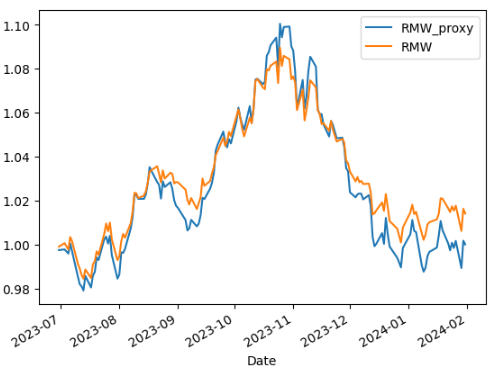
- (basket_hml.big_high + basket_hml.big_low + basket_rmw.big_robust + basket_rmw.big_weak + basket_cma.big_conserv + basket_cma.big_aggress))We can now compare the computed proxy timeseries with official FF timeseries.
comp_rmw = pd.merge(ff_proxy.RMW_proxy[:last_ff_date], data_ff.RMW[cutoff_date:]/100, how='left', left_index=True, right_index=True).dropna()
corr_rmw = comp_rmw.corr().iloc[0,1]
beta_rmw = (comp_rmw.cov() / comp_rmw.RMW.var()).iloc[0,1]
(1+comp_rmw).cumprod().plot()
| Factor | Correlation versus FF Factor | Beta versus FF Factor |
| Mkt-RF | 99.52% | 1.00 |
| SMB | 98.28% | 1.11 |
| HML | 92.46% | 0.85 |
| RMW | 93.92% | 1.16 |
| CMA | 89.77% | 0.95 |
We have pretty good correlations versus the original FF5 factors (as we did not do much refinement on data filtering). We just have to adjust for leverage (i.e. beta) to correctly scale our proxies.
ff_proxy_adjusted = ff_proxy.copy()
ff_proxy_adjusted["MKT_proxy"] = ff_proxy_adjusted["MKT_proxy"] / beta_mkt
ff_proxy_adjusted["HML_proxy"] = ff_proxy_adjusted["HML_proxy"] / beta_hml
ff_proxy_adjusted["SMB_proxy"] = ff_proxy_adjusted["SMB_proxy"] / beta_smb
ff_proxy_adjusted["CMA_proxy"] = ff_proxy_adjusted["CMA_proxy"] / beta_cma
ff_proxy_adjusted["RMW_proxy"] = ff_proxy_adjusted["RMW_proxy"] / beta_rmw
To test the quality of our proxies, we can upload a US index timeseries that we will regress against our 2 factor sets.
# we load an index total return timeserie
index_usa = pd.read_csv("index_usa.csv")
index_usa.dte_Date = pd.to_datetime(index_usa.dte_Date, format="%Y-%m-%d")
index_usa = index_usa.set_index("dte_Date")

start_date = "2023-06-30"
end_date = "2024-01-31"

print("REGRESS AGAINST FAMA FRENCH")

y_ff = index_usa[start_date:end_date]
X_ff = data_ff.drop(columns=["RF"])[start_date:end_date]
y_ff = y_ff[y_ff.index.isin(X_ff.index)]
X_ff = X_ff[X_ff.index.isin(y_ff.index)]
model_ff = sm.OLS(y_ff, sm.add_constant(X_ff/100))
res_ff = model_ff.fit()
print(res_ff.summary())

print("REGRESS AGAINST FAMA FRENCH PROXY")

y = index_usa[start_date:end_date]
X = ff_proxy_adjusted.drop(columns=["RF"])[start_date:end_date]
y = y[y.index.isin(X.index)]
X = X[X.index.isin(y.index)]
model = sm.OLS(y, sm.add_constant(X))
res = model.fit()
print(res.summary())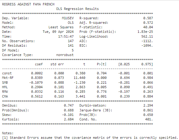
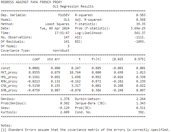
We got pretty similar results, near R² scores and close estimated betas.
Now we can check if the residuals are close too.
res_ff.resid.plot()
res.resid.plot()

comp_resid = pd.merge(res_ff.resid.rename("ff"), res.resid.rename("proxy"), how="inner", left_index=True, right_index=True)
print("corr: ", comp_resid.corr().iloc[0,1])
print("beta: ", (comp_resid.cov() / comp_resid.ff.var()).iloc[0,1])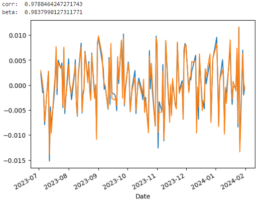
Correlation is near 98%!
To conclude, we denoised quite similarly the index timeseries with both proxy and FF factor sets. We can therefore use these proxy factors to fill in the missing data over 2 months. This will allow us to use this factor model for live investing/trading models. Free data here does not degrade much modeling performance.