Practical implementation of bets on a Strategic Allocation thanks to Black-Litterman approach
As a portfolio manager or as a portfolio construction analyst, the most usual way to manage a fund is to elaborate a Strategic Asset Allocation (a.k.a. “SAA”), that is reviewed on a mid or low frequency, on which PM or researchers add their tactical views, i.e. a Tactical Asset Allocation (a.k.a. “TAA”), which can be refreshed on a higher frequency.
The SAA reflects the long term view of the management team on the different assets, while the TAA allows to implement short-term views and adds a tilt to SAA, hopefully adding some alpha to the fund.
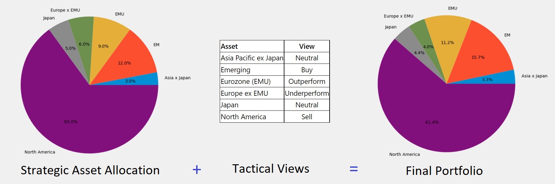
It is the combination of the SAA and the TAA that forms the final portfolio.
This framework allows the portfolio manager to monitor and distinguish the fund’s performance on both long-term allocation and tactical adjustments skills.
Here we will focus on a methodology to implement the TAA tilt, and answer the following questions.
- How should we implement the bets?
- How much weights should we allocate to them?
The model
One solution, well-known, is the Black-Litterman approach. However, for the connoisseurs, it is a model that can be hard to fine-tune as it is very sensitive to parameters’ choices.
The original model talked about absolute or relative views, like an Asset A that should do +5%, or an Asset B that should out-perform some asset C by 3%. In practice this is really hard to predict and to assess.
The most practical way to build our views is with a classification approach, like brokers’ recommendations, we tag an asset as a buy or a sell. We can establish the following classification and rating scale:
| Label | Score |
| Sell | -2 |
| Under-perform | -1 |
| Neutral | 0 |
| Out-perform | +1 |
| Buy | +2 |
Now let’s dig into the model. We are building an “absolute” version of the BL approach.
We have the following starting hypotheses:
An\ asset\ vector\ x , \\ a\ return\ vector\ \bar\mu, \\ a\ volatility\ vector\ \sigma, \\ a\ covariance\ matrix\ \Sigma, \\ a\ risk\ free\ rate\ rf, \\ a\ given\ strategic\ portfolio\ x_{strat} The implied expected returns are the following:
\tilde{\mu} = rf + SR_{x_{strat}}\ \frac{\Sigma\ x_{strat}}{\sqrt{ x_{strat}^\top \Sigma\ x_{strat} }}  \\
\newline
{} \\
with SRx_strat representing the Sharpe Ratio of the SAA:
SR_{x_{strat}} = \frac{x_{strat}^\top \ \bar\mu\ -rf}{ \sqrt{ x_{strat}^\top \Sigma\ x_{strat} } }We build a tactical Sharpe Ratio SRviews, representing our active views, with δ a scaling factor to TAA, v the vector of tactical views and S the rating scale vector.
SR_{views} = \delta\ \frac{v}{n_s} \\
with\ n_s = \frac{-1 + card\ S}{2}
Then we can compute our conditional expected returns:
\breve{\mu} = (SR_{implied} + SR_{views})\  \sigma \\
= \tilde{\mu}+ SR_{views}\  \sigma\ \  \ \\
{}
\newline

where\ SR_{implied} = \frac{\tilde{\mu} - rf}{\sigma} \\
Now we can merge our implied and conditional expected returns to get our final expected returns:
\mu = \frac{\tau}{\tau+1}\ \tilde{\mu}\ +\ (1-\frac{\tau}{\tau+1})\ \breve{\mu} with τ, being our views’ confidence parameter. When we increase τ, we lower the confidence in our views.
The optimization process
Now that we computed our final expected returns, that merged our SAA positioning with our Tactical views, we can focus on portfolio construction, i.e. implementing the bets.
We want to find the optimal portfolio x* with respect to a strategic portfolio (SAA), i.e. maximize expected return while minimizing the risk taken. Also, in order to have a robust portfolio we have to introduce some penalties to control for tactical views impact and turnover . Consequently, we will be using the following convex optimization problem:
x^*\ =\argmin\ \{  \ x_{rel}^\top \Sigma\ x_{rel} - \gamma x_{rel}^\top \mu\ + L_2+ L_1 \}\\
w.r.t:  \sum x = 1 \\
{}
\newline
with: \begin{cases}
x_{rel}  = x - x_{strat} \\
L_2 = (x-x_{strat})^\top \Lambda_1\ (x-x_{strat}),\\
\Lambda_1 =  \lambda_1\ diag(\Sigma)\\
L_1 = \|x-x_{strat}\|_{_1}^\top\ \Lambda'_1,\\
\Lambda'_1 = \lambda'_1 \\
\end{cases} \\
with γ the risk aversion coefficient and L1 and L2 being penalization terms. L1 controlling for the turnover of the resultant portfolio (transaction cost of λ‘1), and L2 smoothing the effects of tactical views on the SAA, acting as a covariance shrinkage factor (λ1).
Practical example
Let’s imagine we have the following equity assets and the associated SAA (which is also the current portfolio):
| Asset | Weight |
| Asia Pacific ex Japan | 3% |
| Emerging | 12% |
| Eurozone (EMU) | 9% |
| Europe ex EMU | 6% |
| Japan | 5% |
| North America | 65% |
Our research team has some short-term views on these assets. Let’s say they have several models and the aggregated views are the following:
| Asset | View |
| Asia Pacific ex Japan | Neutral |
| Emerging | Buy |
| Eurozone (EMU) | Outperform |
| Europe ex EMU | Underperform |
| Japan | Neutral |
| North America | Sell |
The investment committee is quite confident with its views, so they agreed for a risk budget of 50bps (vs SAA).
From these views, we will apply the model we described above, and optimize our portfolio.
Let’s code it!
import pandas as pd
import numpy as np
import cvxpy as cvx
We have our assets input data stored in 3 variables:
- mu_matrix (6×1), estimation of annualized assets returns
- sigma_matrix (6×1), estimation of annualized assets volatilities
- cov_matrix (6×6), estimation of assets covariance matrix
Now we write our use case inputs:
risk_free = 0.02 # risk free rate of 2%, i.e. the current 1M US Treasury rate
ptf = pd.DataFrame(index=data_perf.columns, columns=['Strategic', 'Tactic', 'Portfolio', 'View'], data=0) # the portfolio dataframe
ptf.Strategic = [0.03, 0.12, 0.09, 0.06, 0.05, 0.65] # assets order: ASIA, EM, EMU, EUR, JPY, NAM
ptf.View = [0, -2, 1, -1, 0, 2] # implementing our views
view_scale = [-2,-1,0,1,2] # scaling of views, based on our classification table
tau = 1 # views' confidence parameter
delta = 1 # tactical scale factor
n_s = (-1 + len(view_scale)) / 2 # views normalizer
We chose a τ of 1, this means that our expected returns are equally mixed (50/50) between implied views and tactical views.
We compute our expected returns:
strat_sharpe = ((ptf.Strategic.values @ mu_matrix) - risk_free) / np.sqrt(ptf.Strategic.values.T @ cov_matrix @ ptf.Strategic.values) # sharpe ratio of strategic allocation (SAA)
implied_mu = risk_free + strat_sharpe * (cov_matrix @ ptf.Strategic.values) / np.sqrt(ptf.Strategic.values.T @ cov_matrix @ ptf.Strategic.values) # implied expected return
active_sharpe = delta * ptf.View / n_s # tactical sharpe
conditional_return = implied_mu + active_sharpe * sigma_matrix # conditional expected return based on views
expected_return = (tau/(tau+1)) * implied_mu + (1-(tau/(tau+1))) * conditional_return # incorporate tactical views with strategic implied return
We can now use these expected returns in our optimization process:
gamma = 1 # risk aversion

# Create variables
w_ref = ptf.Strategic.values # strategic allocation
n = len(w_ref) # universe length
w = cvx.Variable(n, pos=True) # optimal weights to find

# Write optimization terms
active_ret = (expected_return.values-risk_free) @ (w-w_ref) # active expected return term
active_risk = cvx.quad_form(w-w_ref, cov_matrix.values) # active risk term

# Choose parameters of regularization terms
lambda_1 = 38 # smoothing parameter, control for active risk
lambda_1_prime = 0.001 # transaction penalty

# Write regularization terms
L_2 = cvx.quad_form(w-w_ref, lambda_1 * np.diag(cov_matrix) * np.eye(n))
L_1 = cvx.norm1(w-w_ref).T * lambda_1_prime

# Write optimization problem and constraints
constraints = [cvx.sum(w) == 1.0]
objective = cvx.Minimize(active_risk - gamma * active_ret + L_2 + L_1)
prob = cvx.Problem(objective, constraints)
prob.solve(verbose=False, solver='CVXOPT')
Here we took 10bps as an average transaction cost for the λ‘1 penalty and we targeted a λ1 penalty of 38 which was equivalent to constrain our portfolio to an active risk of around 50bps vs SAA.
Finally we export our results:
ptf.Portfolio = w.value # store results in dataframe
ptf.Tactic = ptf.Portfolio - ptf.Strategic

result_df = pd.DataFrame(index=['Strategic (SAA)', 'Tactic (TAA)', 'Portfolio'], columns=['Volatility Contrib.', 'Expected Return Contrib.', 'Tracking Error vs SAA'], data=0)

result_df.loc['Portfolio','Tracking Error vs SAA'] = np.sqrt(ptf.Tactic.T.dot(cov_matrix).dot(ptf.Tactic))
result_df.loc['Portfolio','Volatility Contrib.'] = np.sqrt(ptf.Portfolio.T.dot(cov_matrix).dot(ptf.Portfolio))
result_df.loc['Strategic (SAA)','Volatility Contrib.'] = np.sqrt(ptf.Strategic.T.dot(cov_matrix).dot(ptf.Strategic))
result_df.loc['Tactic (TAA)','Volatility Contrib.'] = result_df.loc['Portfolio','Volatility Contrib.'] - result_df.loc['Strategic (SAA)','Volatility Contrib.']
result_df.loc['Portfolio','Expected Return Contrib.'] = (expected_return.values-risk_free) @ ptf.Portfolio
result_df.loc['Strategic (SAA)','Expected Return Contrib.'] = (expected_return.values-risk_free) @ ptf.Strategic
result_df.loc['Tactic (TAA)','Expected Return Contrib.'] = result_df.loc['Portfolio','Expected Return Contrib.'] - result_df.loc['Strategic (SAA)','Expected Return Contrib.']

print(result_df)| Volatility Contrib. | Expected Return Contrib. | Tracking Error vs SAA | |
| Strategic (SAA) | 15.76% | 2.21% | – |
| Tactic (TAA) | 0.07% | 0.83% | – |
| Portfolio | 15.83% | 3.04% | 0.50% |
print(ptf)| Strategic | Tactic | Portfolio | View | |
| Asia ex Japan | 3% | 0.32% | 3.32% | 0 |
| Emerging | 12% | 3.75% | 15.75% | 2 |
| EMU | 9% | 2.15% | 11.15% | 1 |
| Europe x EMU | 6% | -2.00% | 4.00% | -1 |
| Japan | 5% | -0.64% | 4.36% | 0 |
| North America | 65% | -3.58% | 61.42% | -2 |
Ok, so we have a tactical overlay that adds 7bps of volatility and that costs us 50 bps of risk versus SAA. If our views are correct it should add 83 bps of extra returns vs SAA.
If we look at the tactical allocation, it is coherent with the views we have provided with respectively a stronger UW/OW on North America and Emerging stocks.
We now have our final portfolio! We were able to implement our bets and control for their sizing.
References
- Black, F. and Litterman, R.B. (1992), Global Portfolio Optimization, Financial Analysts Journal, 48(5), pp. 28-43.
- Bourgeron, T., Lezmi, E., and Roncalli, T. (2018), Robust Asset Allocation for Robo-Advisors, SSRN, www.ssrn.com/abstract=3261635.